Final Report (For judges)
Summary
In this project, we plan to implement the parallel alternating least squares algorithm for large-scale recommendation, for which the description of the algorithm is described in this paper. We optimize the algorithm from three layers: 1) linear algebra operation; 2) OpenMP for single machine optimization; 3) MPI for communication between machines. For some operations in the linear algebra operations, our implementation is faster than uBlas and some are even than OpenBlas. We also try to make use of Xeon Phi to accelerate it. We make use of conjugate gradient to solve the linear equation in this algorithm. The implementation with the optimized linear algebra operations, is 33x speedup over the implementation with uBlas. With OpenMPI and MPI, more speedup is gained, please refer to the experiment part. The code can be obtained from https://github.com/fishbone/parallelcf.git
Background
Usually, for a recommendation system, it tries to give the prediction for the rating of an item for a user. The method given in the paper tries to solve the problem using the inner product of the embedding vectors of a given user and item. In particular, we represent each user with a dense vector $u_i$ and each item with another dense vector called $v_j$. Then the model predicts the rating that user $i$ will give to item $j$ by taking the inner product of the two vectors: $r_{i,j} = u_i^T v_j$. Assuming we have an matrix with $N$ user and $M$ items and $S$ denotes the set where if pair $(i,j)$ is in the set, we have a observed rating for user $i$ to movie $j$. Then, the objective of the algorithm is to solve the following problem: $$\sum_{i=1}^N \sum_{j=1}^M I((i,j) \in S)(r_{i,j} - u_i^T v_j)^2$$ where $I$ is the indicator function. The parameters we are trying to learn is all the $u$ and $v$ to minimize the differences between the prediction and the actual observed ratings. Note that even though $N$ and $M$ could be large, $u$ and $v$ can lie on some low-dimensional space so as to reduce the computational complexity. Alternating-least-square solves this problem by solving a sequence of least-square subproblems. The reason is that if we fix all the $u$, then the problem is essentially a least-square problem in $v$ and vice versa. Each step should decrease the objective so the algorithm is guaranteed to find a estimate of the parameters.
To be more specific, in ALS every iteration, we first update $U = {u_1,…u_N}$ while fixing $V={v_1,…,v_M}$ to minimize the above loss function, and the global solution of this subproblem is: $$ u_i = (V^T_{j, (i,j) \in S}V_{j, (i,j) \in S})^{-1}V^T_{j, (i,j) \in S}R_{j,(i,j) \in S} $$ for $i=1,…N$. The update rule for $V$ is the same.
Divide it
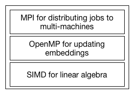
According to the figure above, we divide the optimizations into three layers. The top one is the MPI layer. We want to use MPI to run the algorithm on multiple machines. The middle layer is the OpenMP. With OpenMP, we can reduce the cost of communication between processors, which can't be avoided in MPI. And the lowerest layer is SIMD for optimizing the linear algebra operation.
MPI layer
Since the updating of each user and movie is independent, we can do the calculation in parallel in different nodes. Here the basic idea is that every node is responsible for updating a pre-allocated group of users and movies and after the updating, they will synchronize with each other to the the newest embedding data. Only the movies rated by the assigned users on a single node are stored in the memory for accessing. Here is the flowchart: 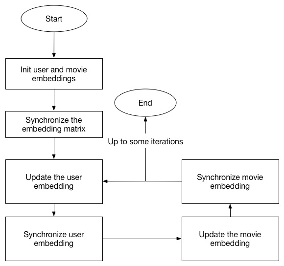
To make things easier to understand, here is the connection and the data assigned in each node:
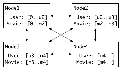
We can see that here there are four nodes, each one stores a pre-allocated part of user embedding and movie embedding. Before updating the embedding of users, the embedding of movies will be synchronized and vice versa.
OpenMP layer
OpenMP layer is very easy. Since we have so many users and movies, we don't want to divide the job into too small granularity. Since the updating of the individual user embedding is independent with others, we can simply just parallelize this section.
SIMD layer
Here there are several linear algebra operations needed to be implemented, which are:
- $M = AA^T$
- $\vec{y} = A\vec{x}$
- $y = \vec{a}^{\,T}\vec{b}$
- $M = A^{-1}$
- $M = A^T$
- $\vec{z} = \vec{x} + \vec{y}$
Most of the operations are optimized by SIMD, except for the inverse operation. Here we'll briefly give the introduction to the method used to optimize them.
Optimizing $M=A^T$
The idea is that firstly we interleave the adjacent rows one by one, and we can get $(a_i,b_i)$, $(c_i,d_i)$, $(e_i,f_i)$, $(g_i,h_i)$ in the same row. And then we interleave odd/even rows with two elements as an unit. After this, we will get $(a_i,b_i,c_i,d_i)$, $(e_i,f_i,g_i,h_i)$ in the same row. For the last step, we interleave row $(0,4)$, $(1,5)$, $(2,6)$, $(3,7)$ with four elements as an unit. After this step, we will get the final results. Here is the figure to illustrate the three steps for this optimizing.
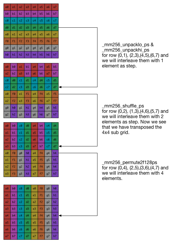
Now we have done the transpose for 8x8 matrix. For a larger matrix, we firstly divide the matrix into 8x8 sub-matrix and transpose each sub-matrix separately.
Optimizing $y=\vec{a}^{\,T}\vec{b}$
Here directly making use of SIMD will help. The idea is that there is a accumulator SIMD vector with initial value as zeros. And divide the input vectors into several segment and multiply the corresponding elements and add to the accumulator vector. After processing all the segments, we sum the value of the accumulator to give the final result. Please refer to the figure below to gain a clearer understanding:
Optimizing $\vec{y}=A\vec{x}$
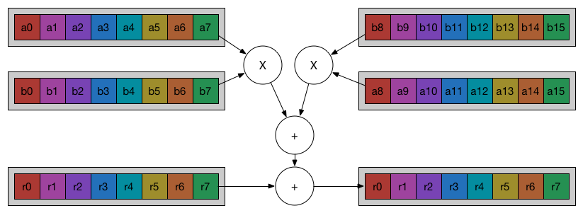
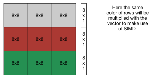
There optimization is straightforward. Since we have AVX2, we can calculate the product of 8x8 with the vector together. The result is a 8x1 vector and we do it for all the 8x8 sub-matrix in the same line and acculumate the sum to the 8x1 vector. Then we get the result.
Optimizing $M=AA^T$
Although it's a matrix matrix production, it's special. So we can do some optimization for this kind of operation.
Firstly, we notice that the result matrix $M$ is symmetric, which means that we only need to calculate half of it and make use of the property to map the calculated data to the other half of the matrix.
Secondly, here the matrix $A$ is stored as row-major order which means that if we want to get $M_{i,j}$, we only need to do dot product with $i_{th}$ row and $j_{th}$ row. There is no need for the pack of the data, because they are on continuous memory address.
Thirdly, we have AVX2, so we can partition the matrix $M$ into several 8x8 small matrices and calculate each one seperately. And then we transpose the calculated sub matrix and map it to the other half. Here OpenMP can be used, because that the calculation of each sub matrix is not that small.
The figure below is to illustrate the process:
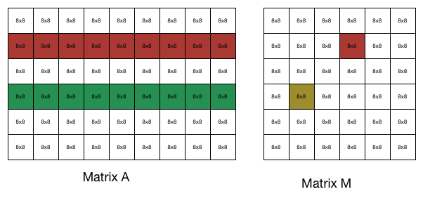
To calculate the red block of matrix $M$, we need to do block dot product with the red row and green row of matrix $A$. This can be done by making use of AVX2. After getting the value of the red block, we can make use of the property of symmetricity to get the value of the yellow block of $M$.
But here comes to another problem: how to parallel calculate the 8x8 sub matrix of $M$? Here one method is to make use of matrix tranpose implemented before, and sum them. But here horizontal sum can be used. See the figure below 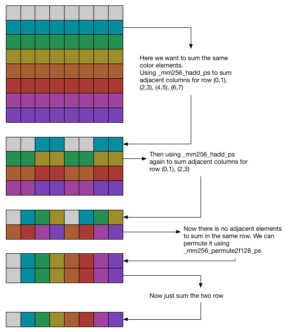 :
:
Firstly, for each continuous row, we use horizontal to sum the adjacent elements. And we can use it again, since there are still some adjacent elements in the results needed to be summed. So we use horizontal sum again. Then we get the $(a,b,c,d,a,b,c,d)$ and $(e,f,g,h,e,f,g,h)$ and we want to sum the elements with the same letter. So we can use the method used in transpose and just sum the two vectors, and we will get the final answer.
Optimizing $M=A^{-1}$
We want to get the inverse of a matrix, because we want to solve a linear equation $A\vec{u}=\vec{v}$ and by getting $A^{-1}$, we can easily get the updated value $\vec{u}$. But here, the only useful value is $\vec{u}$ and in fact we don't care what's $A^{-1}$. So here let's focus on how to get $\vec{u}$. It's easy to notice that the matrix $A$ should be symmetric in this algorithm. So we can employ conjugate gradient to solve this problem.
Here we make use of the primitive operations implemented above to implement this algorithm. Besides, since in every iteration the matrix $A$ will not change too much, we can use the previous value of $u$ as the initial value to make it converge faster.
Experiments
Speedup of linear algebra operations
| Operation | Matrix Dimension | uBlas | OpenBlas | Ours |
|---|---|---|---|---|
| $M=A^T$ | A:100,000x100 | 1.0x | N/A | 3.68x |
| $y=\vec{a}^{\,T}\vec{b}$ | a:10,000 | 1.0x | 4.58x | 7.97x |
| $\vec{y} = A\vec{x}$ | A:100,000x1000 | 1.0x | 2.1214x | 5.3156x |
| $M=AA^T$ | A:128x102400 | 1.0x | 23.4769x | 104.529x |
| $M=AA^T$ | A:1024x1024 | 1.0x | 78.2266x | 102.47x |
| $M=AA^T$ | A:10240x128 | 1.0x | 145.422x | 87.498x |
The speedup is calculated over uBlas library. Here is some analysis for the $M=AA^T$ operation. Because here we calculate by blocks and if the number of columns is small, then each tasks assigned to the thread of OpenMP is relative small (OpenBlas also make use of OpenMP), which increase the overhead of scheduling. And that's why our method is slower than OpenBlas.
Speedup of the whole algorithm
Data Set
The data set here using is from MovieLens 10M and MovieLens 20M.
Testing environment
The experiment here is done in the latedays cluster in CMU, where each node is installed with two, six-core Xeon e5-2620 v3 processors (2.4 GHz, 15MB L3 cache, hyper-threading, AVX2 instruction support).
Compare with uBlas naive implementation
The implementation of uBlas is the one implemented according what's stated in the paper. After the optimizing of the basic linear algebra operations together with conjugate gradient, we easily gain a speed up of 33x on a single machine with only one thread without MPI or OpenMP over the implementation of uBlas. This data is calculated on the data set of MovieLens 10M with the dimension of embedding matrix as 32. It's not a surprising, because from the statistics in the previous section, out implementation is much faster than that of uBlas. What's more, conjugate gradient also helps accelerate. Besides, when optimized with OpenMP using 24 threads, we can gain a speedup of 153x. For the final version, which means that 8 nodes with 24 threads per nodes, the speedup is about 420x.
Speedup of OpenMP and MPI
In this section, we use the optimized linear algebra algorithm and change the number of threads and machines to observe the speedup with this two variables.
Firstly, here is the speedup on single machine with the OMP_NUM_THREADS increase:
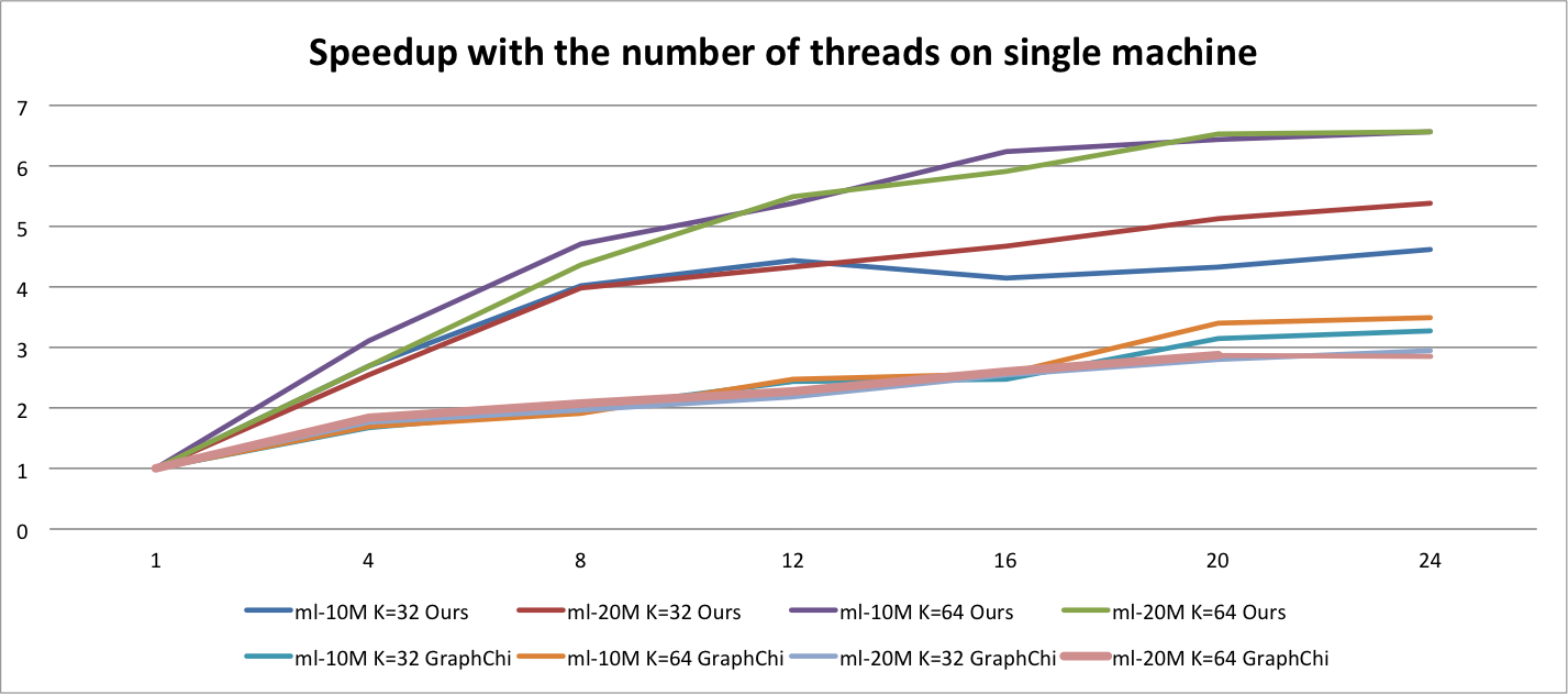
Here the x-axis is the number of threads and the y-axis is the speedup of the one running with only one thread. $K$ is the dimension of embeddings. Since ml-20m data set is bigger that ml-10m which means that more computation is needed. So the speedup of ml-20m is better than that of ml-10m. Besides, we also compare the speedup with the one of GraphChi. For each line of GraphChi it's calculated over the single implementation of GraphChi. And we can see the scalability of our implementation is better than that of GraphChi. Besides, although not shown in the graph, our implementation is much faster than that of GraphChi.
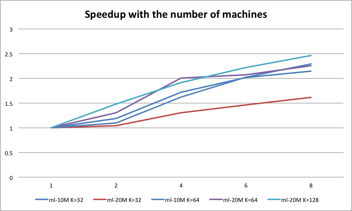
Here the x-axis is the number of machines and the y-axis is the speedup of the one running within one node. Since for MPI, it needs communication between each nodes. For every iteration, it needs to synchronize with other nodes for both the user embeddings and movie embeddings, which means that the larger the dataset is, the more communication will be done. And because ml-20m data set is bigger than ml-10m which require more communication between nodes, the speedup worse than that of ml-10m. Besides, with increasing number of machines, each machine will be responsible for smaller sub set of movies and users, which means that more data will be received from other nodes. So we see that for ml-10M, when the number of machines is greater than 4, the increasing of the speedup is not that significant, and it's also the same for ml-20M. What's more if we increase the dimension of the embedding matrix, the communication cost will not be that important and we can see a higher speedup when the number of machines increase, such as ml-20m K=128
**Finally, the implementation over that of uBlas
In the end we give the graph of the speedup of our final implementation (with OpenMP, SIMD optimization, and MPI) over the one implemented according to the paper with uBlas.
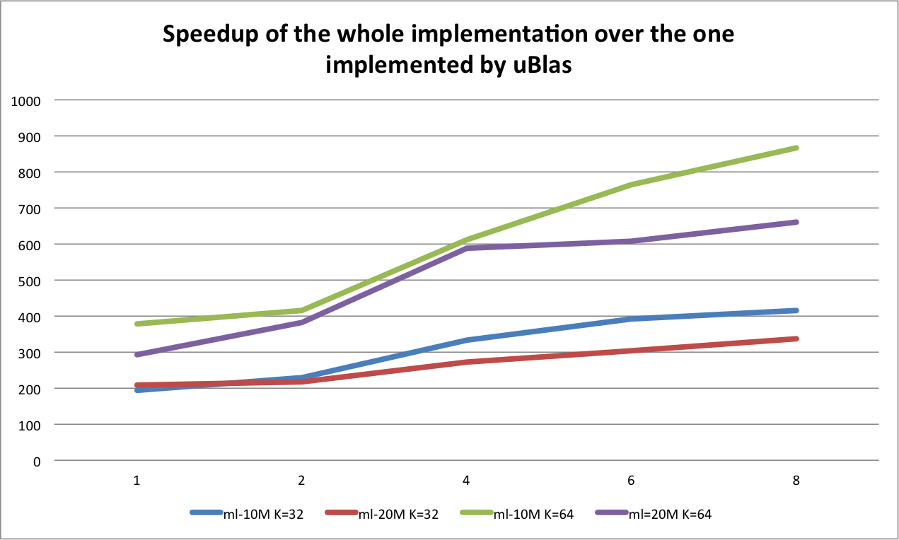 The x-axis is the number of machines and y-axis is the speedup over the implementation with uBlas. Here we can see the speedup is significant. Besides, we can also notice there is some similar conclusions:
- The optimization with SIMD and OpenMP works. Because for all lines, when running on a single machine, the speedup is more than 200x.
- MPI helps more when the dataset is not that big or when the dimension of the embedding matrices is bigger. When the dataset is not big, the communication between nodes is relative small. When the dimension of embedding matrices is bigger, the computation will be more. At this point, the time spending on communication is less than that of computing. More more machines can reduce the time in computation while not increase much in commucation. In the experiment, MPI helps.
The place where can be improved
From the experiment, we can know, the communcation between machines is one of the biggest factor for training on larger dataset. So we need to focus on how to reduce the communication cost by maybe chaning the algorithms described in the paper, which may lead to different but similar performance of the model.